Get full access to Packet Guide to Routing and Switching and 60K+ other titles, with a free 10-day trial of O'Reilly.
There are also live events, courses curated by job role, and more.
The previous book in this series, The Packet Guide to Core Network Protocols, covered the IPv4 protocols, masking, and devices that are part of every network. Now it’s time to take on the routing and switching for the network. There are an astonishing number of table-based decisions that have to be made in order to get a single packet across a network, let alone across a series of networks. Not limited to routers, switches, and access points, these decisions are made at each and every device, including hosts. As networks are constructed and devices configured to forward packets and frames, network administrators must make critical decisions affecting performance, security, and optimization.
When moving to advanced ideas, the net admin should know how and why networking tables are constructed, and in what cases manual changes will be beneficial. This chapter provides details about the routing and switching operations, as well as design elements. This chapter assumes that the reader understands the basic operation of routers and switches, as well as the standard suite of protocols including Ethernet, Internet Protocol (IP), Address Resolution Protocol (ARP), and the Internet Control Message Protocol (ICMP).
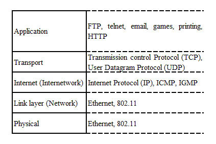
Most protocols are foregone conclusions, so when building networks, many of the choices are not choices at all. It is highly probable that a network will be a mixture of Ethernet and 802.11 nodes. These nodes will run the Internet Protocol at Layer 3 of the Transmission Control Protocol/Internet Protocol (TCP/IP) networking model (see Figure 1-1). The applications will be designed for TCP or the User Datagram Protocol (UDP).
There are many types of switching: packet, circuit, multilayer, virtual circuit, wide area network (WAN), local area network (LAN). Circuiting and virtual circuit switching almost always refer to WAN or telephone technologies, and as such, will not be part of our discussion. Packet switching usually concerns a router or perhaps a WAN switch. Multilayer switching is a technique for improving the processing of IP packets, but most vendors have different ideas as to the best approach. Often, LAN switches are deployed without any thought to how multilayer switching might improve performance. In fact, other than routing between VLANs, administrators are rarely interested in how advanced features might be used on the network. Since this book is about IP-based networking, switching will almost always refer to Ethernet frames and the routing will be that of IP packets.
Switches operate at Layer 2 of the TCP/IP (and OSI) model and are the workhorses of most networks. The operation of switches and bridges is defined in the IEEE 802.1D standard. The standard also describes the behavior of other Layer 2 protocols, such as the Spanning Tree Protocol, which will be covered in Chapter 3.
In network design, we often talk about the “access” layer or how host devices are connected to the network. Switches and access points (we’ll ignore the use of hubs and collision domains) cover all of the bases. In addition to forwarding Ethernet frames based on Media Access Control (MAC) addresses and processing the Cyclical Redundancy Check (CRC), switches provide a couple of very important services:
Switches also provide a collection of features that are part of most medium and large networks:
Any device connected to a network, regardless of its specialization, still has to follow the rules of that network. Thus, switches still obey the rules for Ethernet access and collision detection. They also go through the same auto-negotiation operations that Ethernet hosts complete. There are several different link types used when installing switches. They can be connected directly together in point-to-point configurations, connected to shared media or to hosts. Depending on the location in the network, the requirements for performance and security can be significantly different. Core or backbone switches and routers may have the requirement of extremely high throughput, while switches connected to critical elements may be configured for stricter security. Many switches have absolutely no configuration changes, and are simply pulled out of the box and run with default factory settings.
To forward or filter Ethernet frames, the switch consults a source address table (SAT) before transmitting a frame to the destination. The SAT is also called a MAC address table or content addressable memory (CAM). Only the destination indicated in the table receives the transmission. In general, a switch receives a frame, reads the MAC addresses, performs the Cyclical Redundancy Check (CRC) for error control, and finally forwards the frame to the correct port. Broadcast and multicast frames are typically forwarded everywhere except the original source port. Figure 1-2 depicts a typical topology with a switch at the center.

Network nodes have unique MAC addresses and Ethernet frames indentify the source and destination by these MAC addresses. A MAC address is a 6-byte value, such as 00:12:34:56:78:99 , which is assigned to the host. The SAT is a mapping between the MAC addresses and the switch ports. This table also keeps track of the virtual local area networks, or VLANs, configured on the switch. On most switches, all ports are in VLAN 1 by default. The source address table for the network shown in Figure 1-2 might look like Table 1-1.
If the address is known, the frame is forwarded to the correct port. If the address is unknown, the frame is sent to every port except the source port. This is called flooding. If the destination MAC address is a broadcast address (in the form ff:ff:ff:ff:ff:ff ), the frame is again sent everywhere except the original source port. In many cases, this is also the behavior for multicast frames. Recall that multicast frames commonly begin with a hexadecimal 01 in the first byte. The range of a multicast frame can be affected by using the Interior Group Management Protocol (IGMP). Switches can perform IGMP snooping in order to determine which ports should receive the multicast traffic. IGMP is also defined in the IEEE 802.1D standard. VLANs can reduce the effect of flooding or broadcasting because they can be used to break the switch into smaller logical segments. We’ll talk about VLANs in Chapter 4.
Figure 1-3 displays the source address table from an operating Cisco switch. This output was obtained using the show mac-address-table command for the Cisco switch. The term “dynamic” means that the switch learned the address by examining frames sent by the attached nodes.
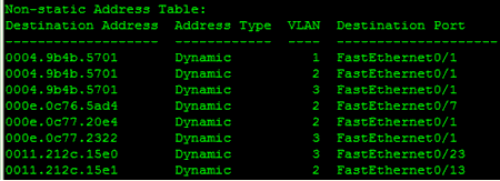
Note that there are three VLANs and port 1 (FastEthernet0/1) has several associated MAC addresses. This is because another switch was connected at that point. An example of this type of topology in shown in Figure 1-4. Two switches are interconnected via Port 3 on Switch 1 and Port 3 on Switch 2. As normal traffic flows, the switches will learn where all of the MAC destinations are by recording the source MACs from the Ethernet transmissions.
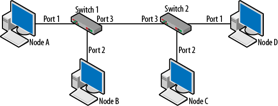
In topologies such as this, it is impossible for a switch to connect directly to each destination. For example, the only piece of information Switch 2 will possess is the source MAC from its perspective. So, from the perspective of Switch 2, all frames appear to have come from the single port (3) connected to Switch 1. The reverse is also true. Building on what is known of source address tables and the learning process, the SATs for the two switches would look like Table 1-2.
When Node A sends traffic to Node D, Switch 1 forwards the traffic out Port 3. Switch 2 receives the frame and forwards the frame to Port 1.
Figure 1-3 also depicts several VLANs. What isn’t clear from these SATs or topology diagrams is how traffic moves from one VLAN to another. Interconnected switches configured with VLANs are typically connected together via trunk lines. In addition, Layer 2 switches need a router or routing functionality to forward traffic between VLANs. With the advent of multiplayer switches, the boundary between routers and switches is getting a bit blurry. VLANs and trunks will be covered in-depth in Chapter 4.
One other very nice feature of a switch is port mirroring. Mirroring copies the traffic from one port and sends it to another. This is important because over the last several years, hubs have been almost entirely removed from the network. But without hubs, it can be a challenge to “see” the traffic that is flowing on the network. With mirroring, a management host can be installed and collect traffic from any port or VLAN. The following are examples of the commands that might be issued on a Cisco switch:
monitor session 1 source interface Fa0/24 monitor session 1 destination interface Fa0/9 encapsulation dot1q
The first command describes the source of the traffic to be monitored. The second command not only specifies the destination, but the type of frame encapsulation as well. In this case, the traffic monitored is actually flowing over a trunk line. Trunks are part of Chapter 4. Mirroring commands can also specify the direction of the desired traffic. It is possible to select the traffic traveling to or from a specific host. Typically, both directions are the default.
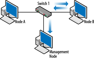
Figure 1-5 depicts an example in which Nodes A and B are communicating and the network admin would like to see what they are up to. So, the traffic coming to and from Node B is mirrored to the management node. Since the conversation is between Node A and B, a port connected to either one of them will suffice.
When building networks, we typically divide routing into two components: host and router. Routers handle traffic flowing between networks but hosts make many decisions long before the packets hit the network. Most routing protocols used to find pathways to destinations are router based, however.
Hosts are typically configured one of two ways: statically with an IP address, default gateway, and domain name server, or with values learned via the Dynamic Host Configuration Protocol (DHCP). Hosts send all traffic going off the local network to the default gateway, with the hope that the gateway can route the packets to the destination. One of my favorite questions to ask is “What is the first thing that a host does before sending a packet?” Before doing anything else, a host must process its routing table. Chapter 2 of this book is devoted to host-based routing. Historically, there have been some network technologies in which the hosts were more active. For example, IBM’s Token Ring utilized discovery frames to find destination nodes on different network segments or rings. However, this is primarily a Layer 2 function, and is not part of contemporary Ethernet- and IP-based networks. Recent years have seen a return to utilizing the host of handling the routing function in the area of ad hoc networking.
Ad hoc routing typically does not run on the traditional network infrastructure. Applications include sensor networks, battlefield communications, and disaster scenarios in which the infrastructure is gone. In these situations, nodes will handle forwarding of traffic to other nodes. Related ideas are the ad hoc applications and 802.11 ad hoc networks. It is important to realize that with the 802.11 standard, nodes can connect in an ad hoc network but do not forward traffic for other nodes. If a wireless node is not within range of the source host, it will miss the transmission.
Ad hoc routing protocols are designed to solve this particular problem by empowering the nodes to handle the routing/forwarding function. Interesting problems crop up when the “router” may not be wired into the network: things such as movement of the wireless nodes, power saving, processing capability, and memory may be affected. In addition, the application is important. Are the nodes actually sensors which have very little in the way of resources? Are they moving quickly? These challenges have resulted in several ad hoc routing protocols being developed, such as Ad hoc On Demand Distance Vector (AODV), Fisheye State Routing (FSR), and Optimized Link State Routing (OLSR).
But these ideas are all a little beyond the scope of this book. The point being made here is that hosts and the host routing table are very active in the processing of packets. Historically, nodes on some networks were even more involved, and if ad hoc routing protocols are any indication, those days are not gone for good.
Routers operate at the internetwork layer of the TCP/IP model and process IP addresses based on their routing table. A router’s main function is to forward traffic to destination networks via the destination address in an IP packet. Routers also resolve MAC addresses (particularly their own) by using the Address Resolution Protocol (ARP). It is important to remember that Layer 2 (link layer) frames and MAC addresses do not live beyond the router. This means that an Ethernet frame is destroyed when it hits a router. When operating in a network, a router can act as the default gateway for hosts, as in most home networks. A router may be installed as an intermediate hop between other routers without any direct connectivity to hosts. In addition to routing, routers can be asked to perform a number of other tasks, such as network address translation, managing access control lists, terminating virtual private network or quality of service.
Basic router functionality is comprised of three major components:
The routing process is the actual movement of IP packets from one port to another and the routing table holds the information used by the routing process. Routing protocols such as the Routing Information Protocol (RIP) or Open Shortest Path First (OSPF) are used to communicate with other routers and may end up “installing” routes in the routing table for use by the routing process. When a router is configured, the routing table is constructed by bringing interfaces up and providing the interfaces with IP addresses. A simple Cisco routing table is shown in Figure 1-6.
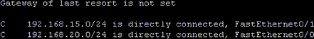
When processing packets, routers “traverse” the routing table looking for the best possible pathway match. The routing table shown in Figure 1-6 indicates that the router knows of two networks: 192.168.15.0 and 192.168.20.0 . Note that this router does not have a default gateway or “gateway of last resort.” This means that if the destination IP address is anywhere beyond the two networks listed, the router has no idea how to get there. If you said to yourself, “Ahh, ICMP destination unreachable message,” give yourself a gold star.
Routing tables can be comprised of several different route types: directly connected, static, and dynamic. Two directly connected routes are seen in Figure 1-6. These are the networks on which the router has an interface and are accompanied by the letter “C” and the particular interface, such as FastEthernet0/1 . Directly connected routes have preference over and above any other route.
The 0/1 from the interface is a designator for the blade and port in the router chassis.
Static entries are those that are manually installed on a router by the network administrator. For specific destinations, and in small or stable network environments, manually configured static routes can be used very successfully. By using static routes, the network administrator has determined the pathway to be used to a particular destination network. The static route will supersede any pathway learned via a routing protocol because of the administrative distance, discussed later in this chapter.
Another important idea that is central to routing is the next hop. The next hop is a router that is one step closer to the destination from the perspective of a particular router. The next hop is the router to send packets to next. In many networks, a series of next hops are used. A medium-sized routed topology is shown in Figure 1-7. So, from the perspective of R1, R2 would be the next hop used to get to both the 192.168.3.0 and 192.168.4.0 networks.
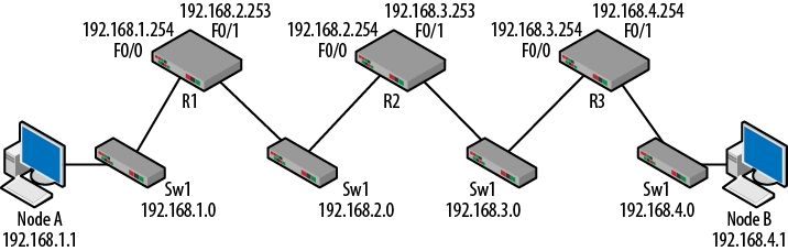
This topology has three routers, which are cabled to each other via the switches shown. There are several ways to emulate a topology such as this, but this configuration was chosen for clarity. Initially, nothing has been configured except that the interfaces have been “brought up” and given IP addresses. To bring up an interface, it has to have been given the no shutdown command and have a link pulse. The routing tables of the routers will only contain the directly connected routes. Each router is only aware of the two networks for which is has interfaces. Table 1-3 depicts the routing tables at this point.
What is clear from these tables is that the routers do not have a complete picture of the whole network. For example, Node A is connected to Switch 1 and is trying to contact Node B on Switch 4. After processing its host routing table (see Chapter 2), it will forward the traffic to its default gateway ( 192.168.1.254 ) on R1. R1 will now consult its routing table and discover that it only has entries for networks on the left side of the topology. Without knowledge of the destination network, R1 will issue the ICMP destination unreachable message.
Just for fun: The 192.168.1.0 and 192.168.4.0 networks are called stub networks because they have only one pathway in or out.
How is this problem solved? In small networks such as this, the network administrator can issue routing commands to the routers providing them with additional forwarding information. These would be the static routes. For Cisco routers, the command ip route is used. It has three fields that have to be filled in by the network administrator:
ip route destination-network destination-network-mask next-hop-IP-address (forwarding router interface)
For example, R1 could be told how to get to the 192.168.3.0 and the 192.168.4.0 networks with the following commands:
ip route 192.168.3.0 255.255.255.0 192.168.2.254 ip route 192.168.4.0 255.255.255.0 192.168.2.254
The commands are almost identical except for the destination network. A couple important points: the last field specifying the forwarding router interface ( 192.168.2.254 ) is a neighboring router that can be reached by R1. With these two commands, the behavior is that from R1 the traffic is destined for the two networks specified should be sent to R2. The mask is also the mask of the destination network and not the mask used locally. It is possible that these masks are different. This correct form is called a recursive route.
After issuing the commands on R1, the routing tables would be updated as listed in Table 1-4: